21Finale: Publication Polish with patchwork, ggrepel & ggtext
In this chapter, we will combine multi-plot layouts (patchwork), collision-free labels (ggrepel) and rich text (ggtext) into three polished before/after case studies.
NoteWhy this matters
Individual plots answer single questions. Combining them into one composed figure with clean labels is what separates an exploratory chart from a published one.
WarningCommon pitfall
Each extension adds load time and new syntax. Master core ggplot2 first; reach for these only for final figures.
21.1 Case 1: Multi-Plot Layout
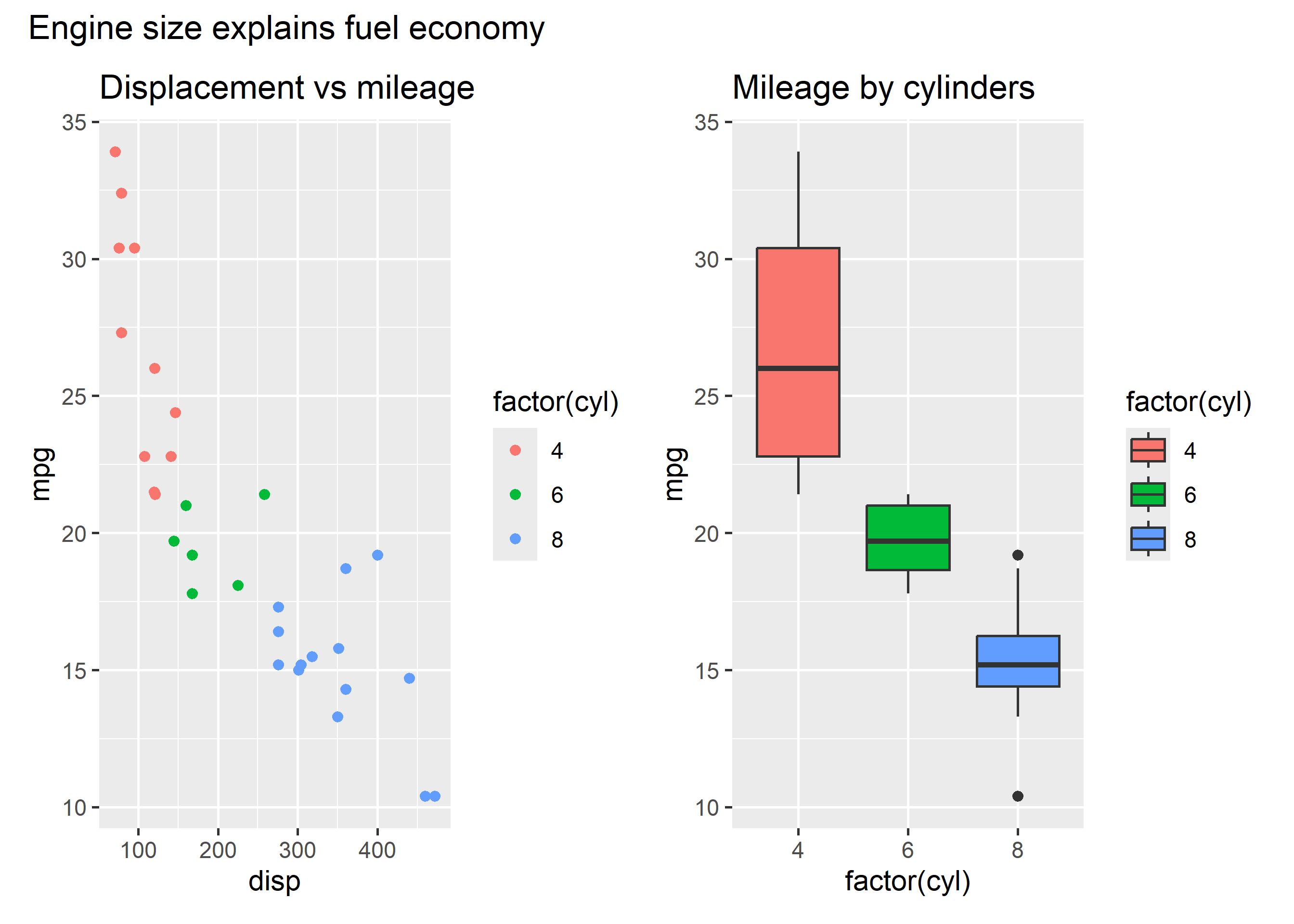
Before: two related plots shown separately. After: one composed figure with a shared title.
p1 <-ggplot(mtcars) +geom_point(aes(disp, mpg, color =factor(cyl))) +labs(title ="Displacement vs mileage")p2 <-ggplot(mtcars) +geom_boxplot(aes(factor(cyl), mpg, fill =factor(cyl))) +labs(title ="Mileage by cylinders")p1 + p2 +plot_annotation(title ="Engine size explains fuel economy")
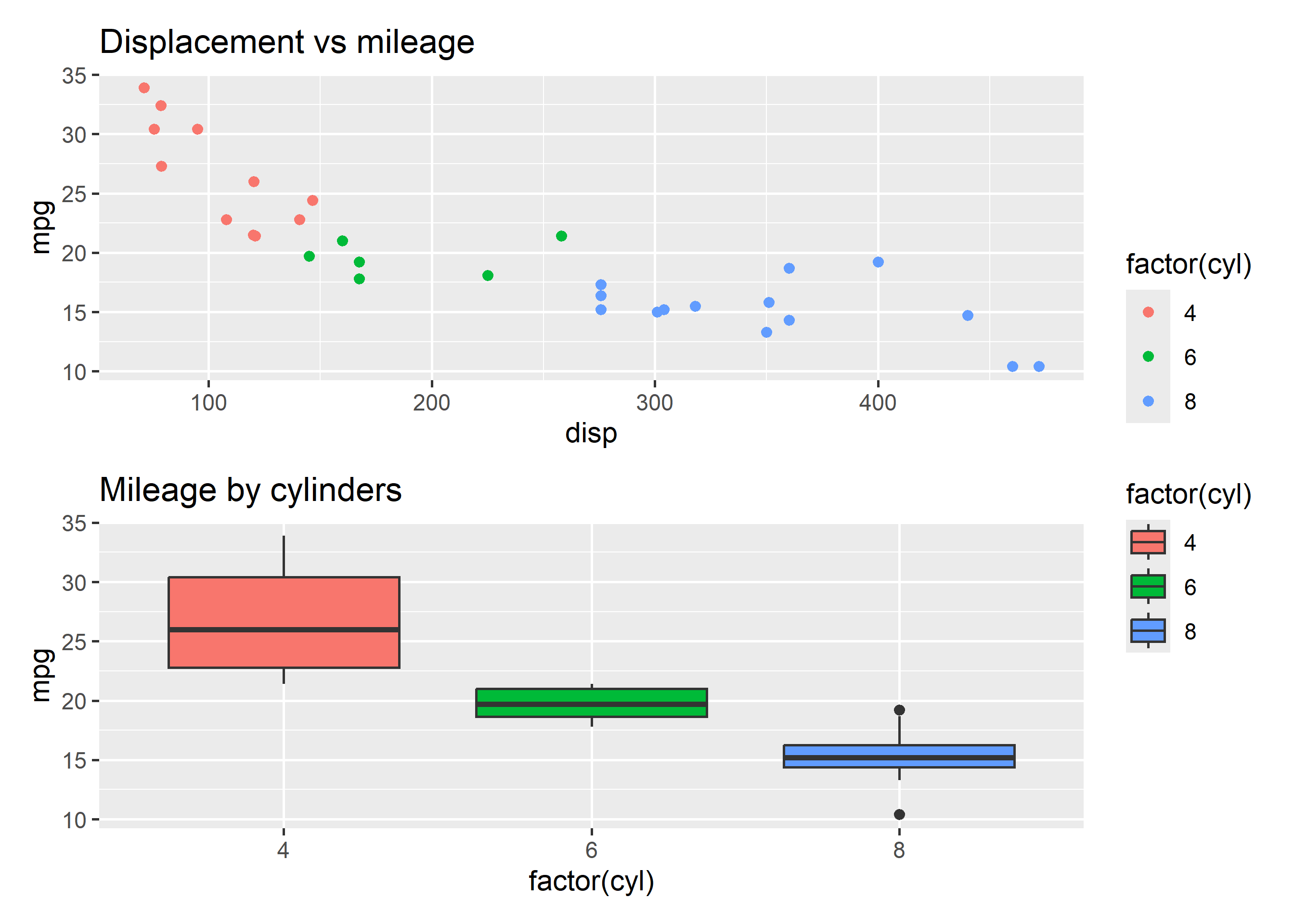
Stack vertically with / and collect legends with plot_layout(guides = "collect"):
p1 / p2 +plot_layout(guides ="collect")
21.2 Case 2: Collision-Free Labels
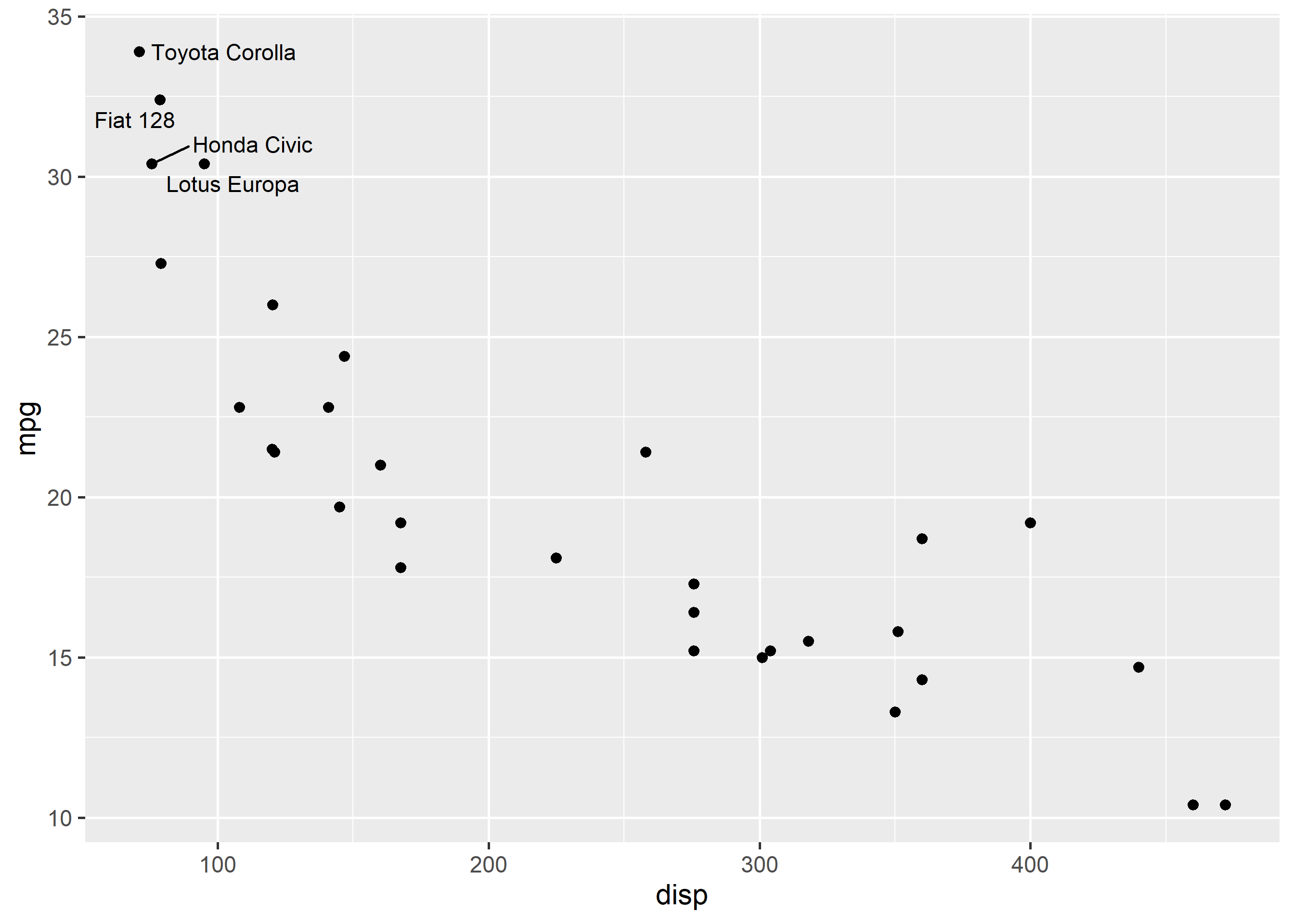
Before: geom_text() labels pile onto each other. After: geom_text_repel() pushes them apart with thin leader lines.