Chapter 14 Themes
14.1 Introduction
In this final chapter, we will learn to modify the appearance of all non data components of the plot such as:
- axis
- legend
- panel
- plot area
- background
- margin
- facets
14.2 Basic Plot
We will continue with the scatter plot examining the relationship between displacement and miles per gallon from the the mtcars data set.
p <- ggplot(mtcars) +
  geom_point(aes(disp, mpg))
p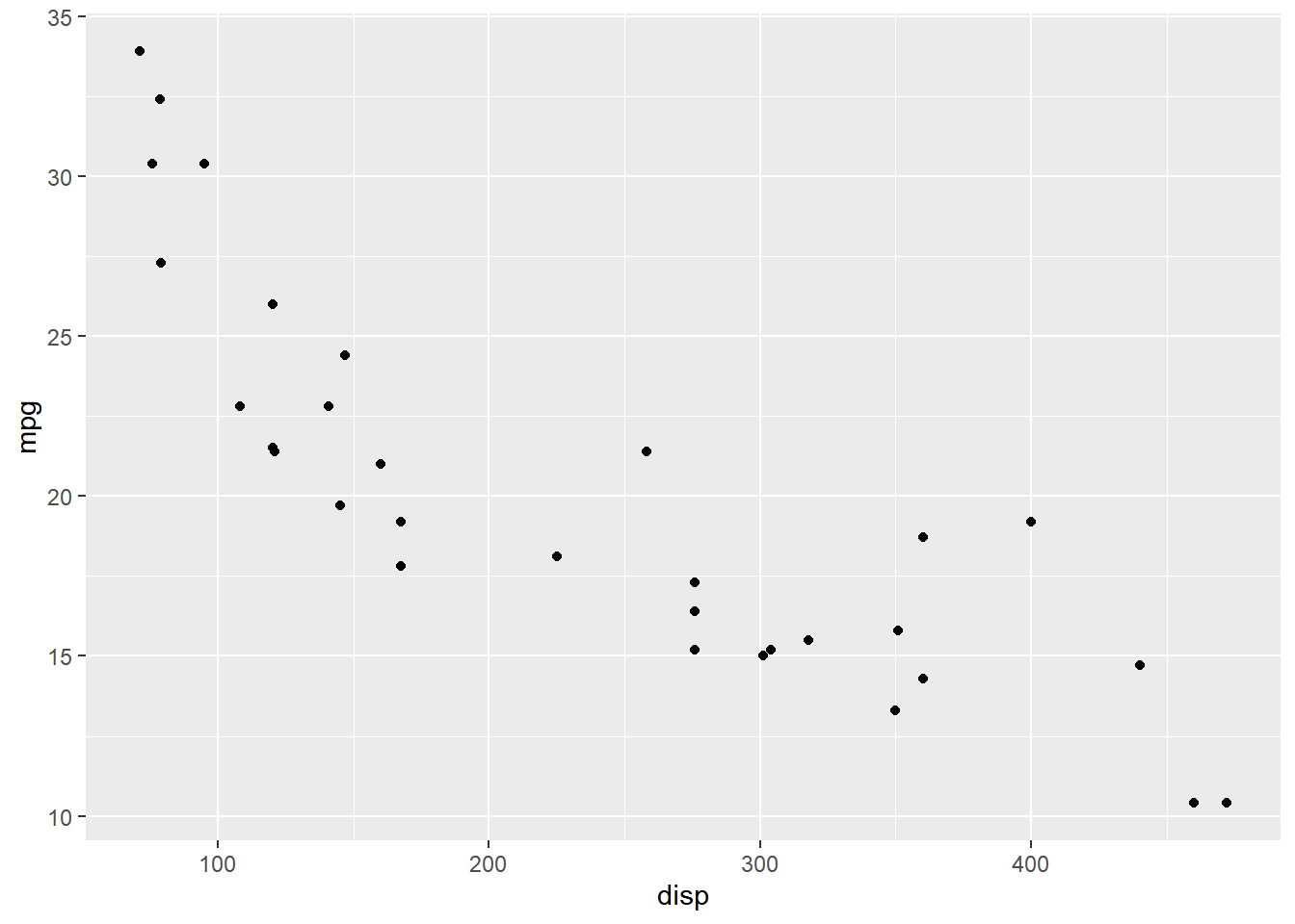
14.3 Axis
14.3.1 Text
The axis.title.x argument can be used to modify the appearance of the X
axis. In the below example, we modify the color and size of the title using
the element_text() function. Remember, whenever you are trying to modify the
appearance of a theme element which is a text, you must use element_text().
You can use axis.title.y to modify the Y axis title and to modify the
title of both the axis together, use axis.title.
p + theme(axis.title.x = element_text(color = "red", size = 10, face = "italic"))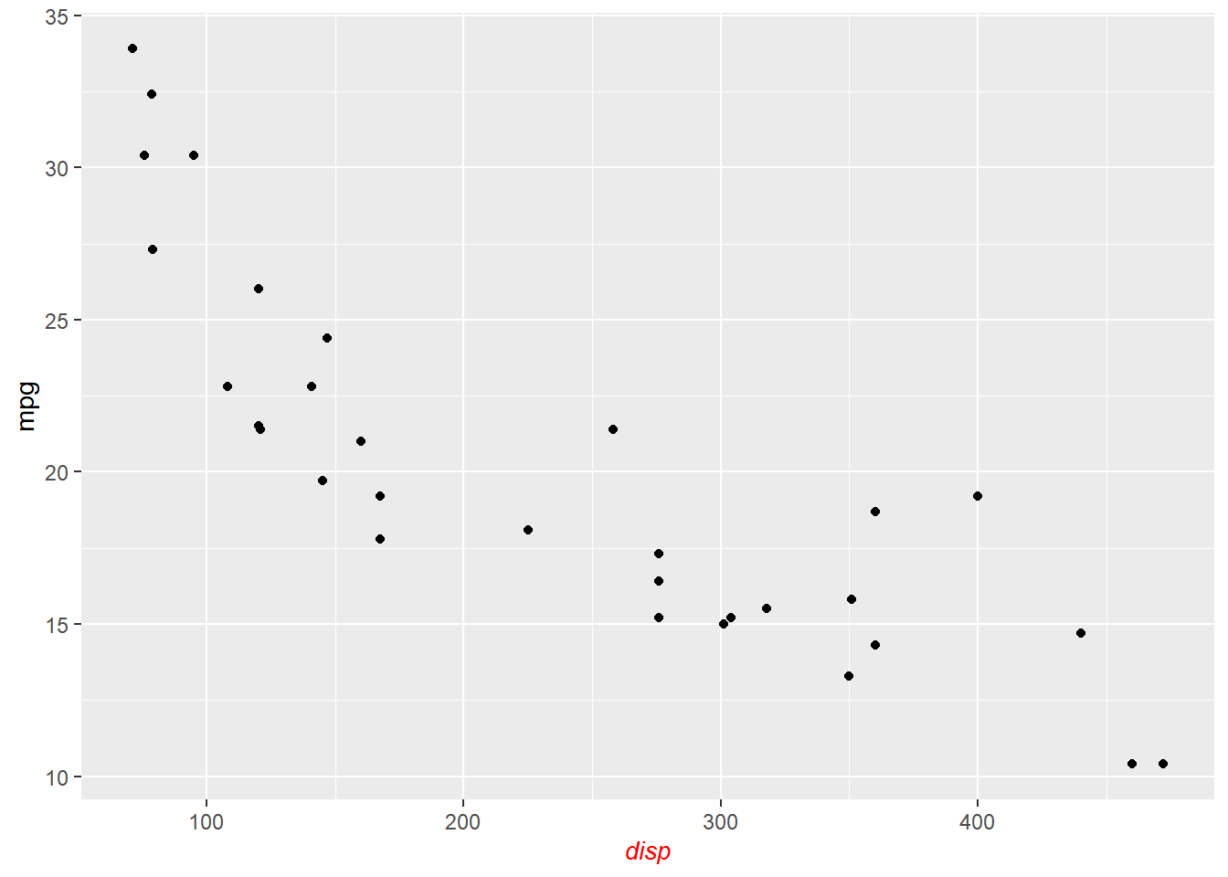
14.3.2 Ticks
To modify the appearance of the axis ticks, use the axis.ticks argument. You can
change the color, size, linetype and length of the ticks using the element_line()
function as shown below.
p + theme(axis.ticks = element_line(color = 'blue', size = 1.25, linetype = 2),
          axis.ticks.length = unit(1, "cm"))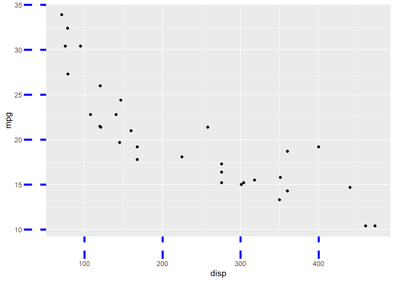
14.3.3 Line
The axis.line argument should be used to modify the appearance of the
axis lines. You can change the color, size and linetype of the line using
the element_line() function.
p + theme(axis.line = element_line(color = 'red', size = 1.5, linetype = 3))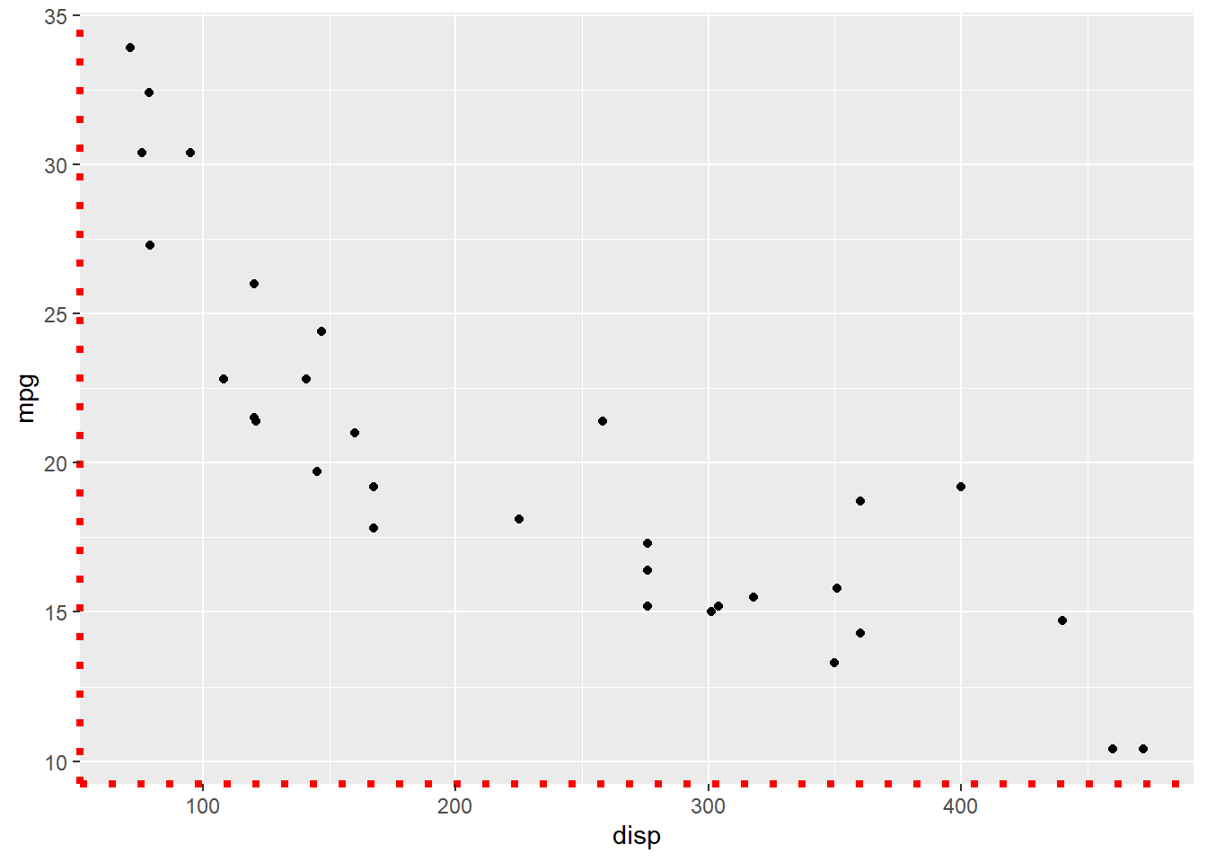
14.4 Legend
Now, let us look at modifying the non-data components of a legend.
p <- ggplot(mtcars) +
  geom_point(aes(disp, mpg, color = factor(cyl), shape = factor(gear)))
p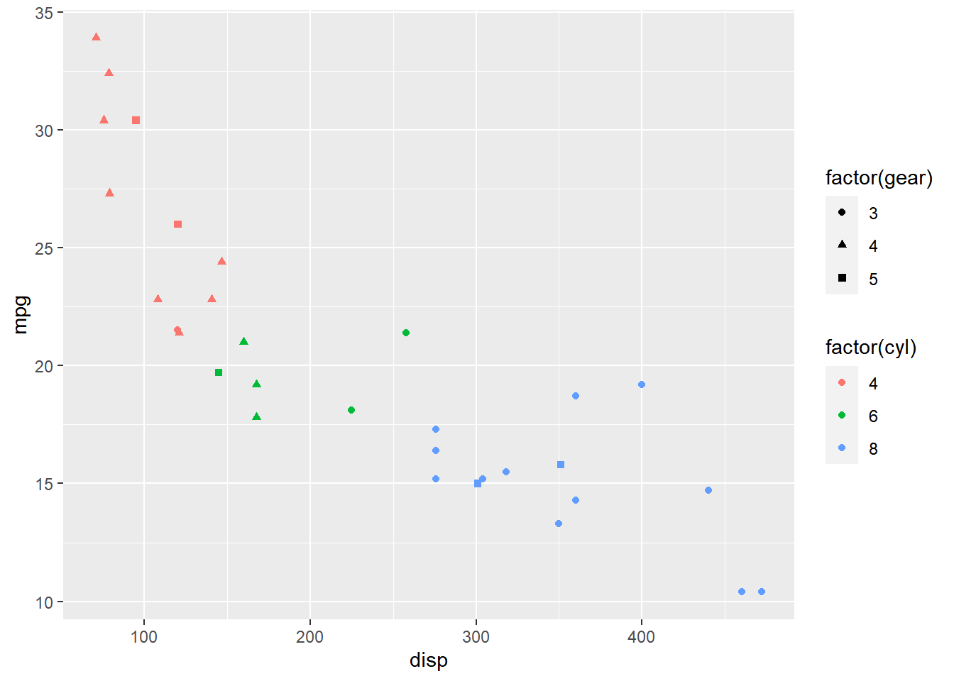
14.4.1 Background
The background of the legend can be modified using the legend.background
argument. You can change the background color, the border color and line type
using element_rect().
p + theme(legend.background = element_rect(fill = 'gray', linetype = 3,
          color = "black"))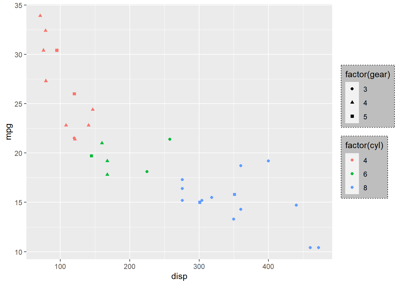
14.4.2 Text
The appearance of the text can be modified using the legend.text argument.
You can change the color, size and font using the element_text() function.
p + theme(legend.text = element_text(color = 'green', face = 'italic'))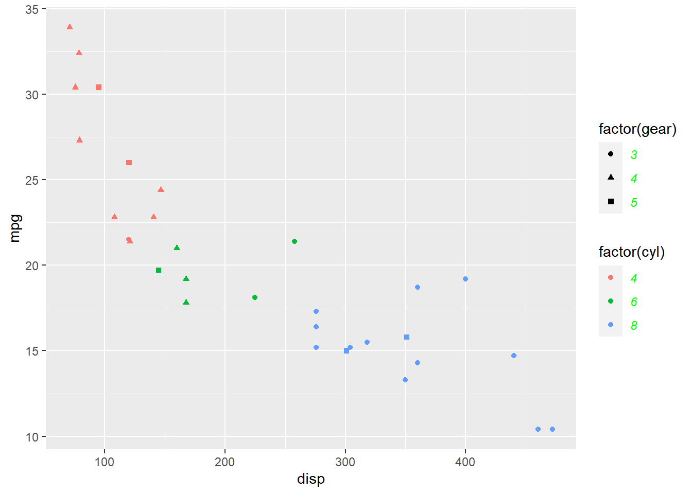
14.4.3 Title
The appearance fo the title of the legend can be modified using the
legend.title argument. You can change the color, size, font and alignment
using element_text().
p + theme(legend.title = element_text(color = 'blue', face = 'bold'),
          legend.title.align = 0.1)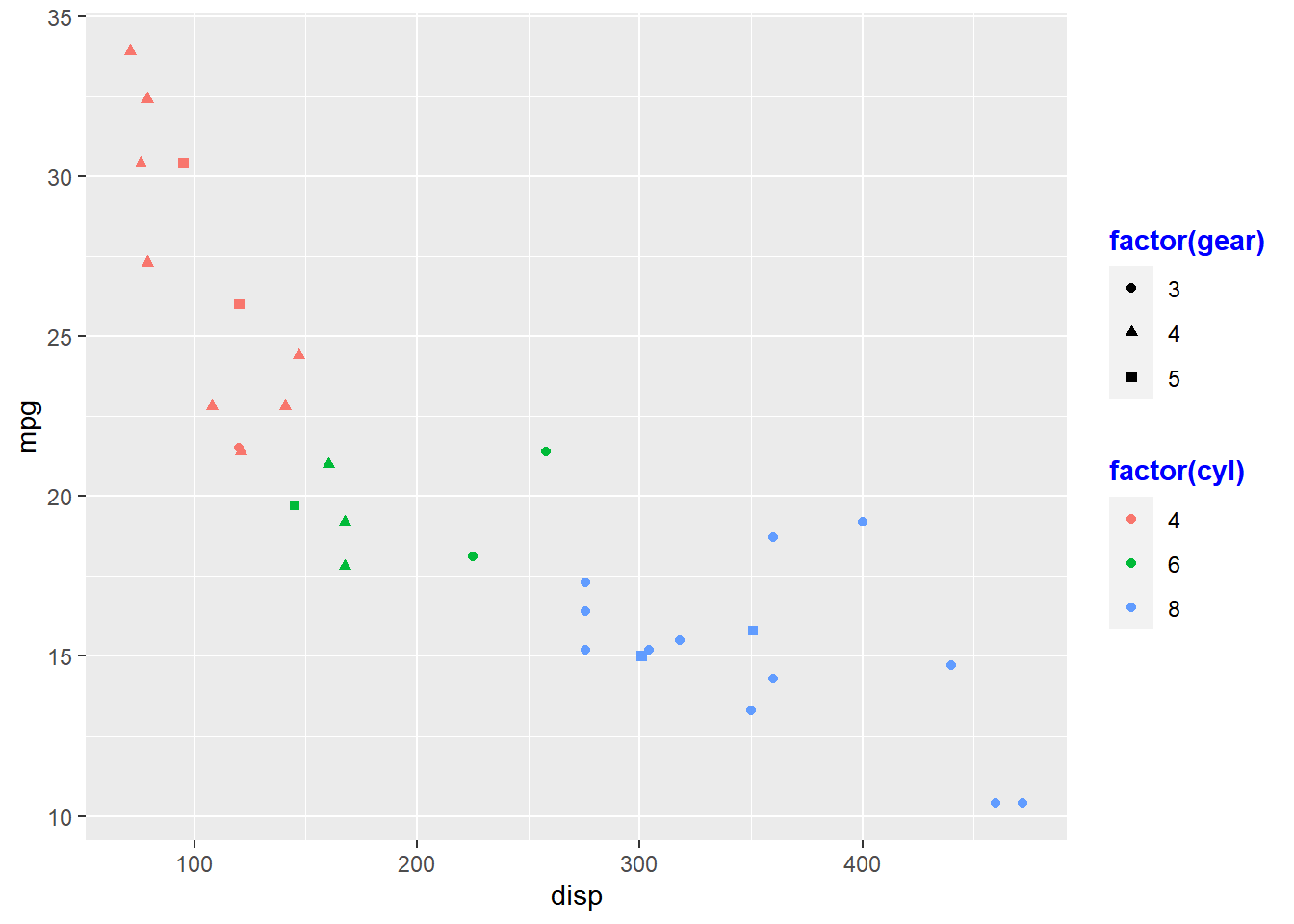
14.4.4 Position
The position and direction of the legend can be changed using:
legend.position- and
legend.direction
p + theme(legend.position = "top", legend.direction = "horizontal")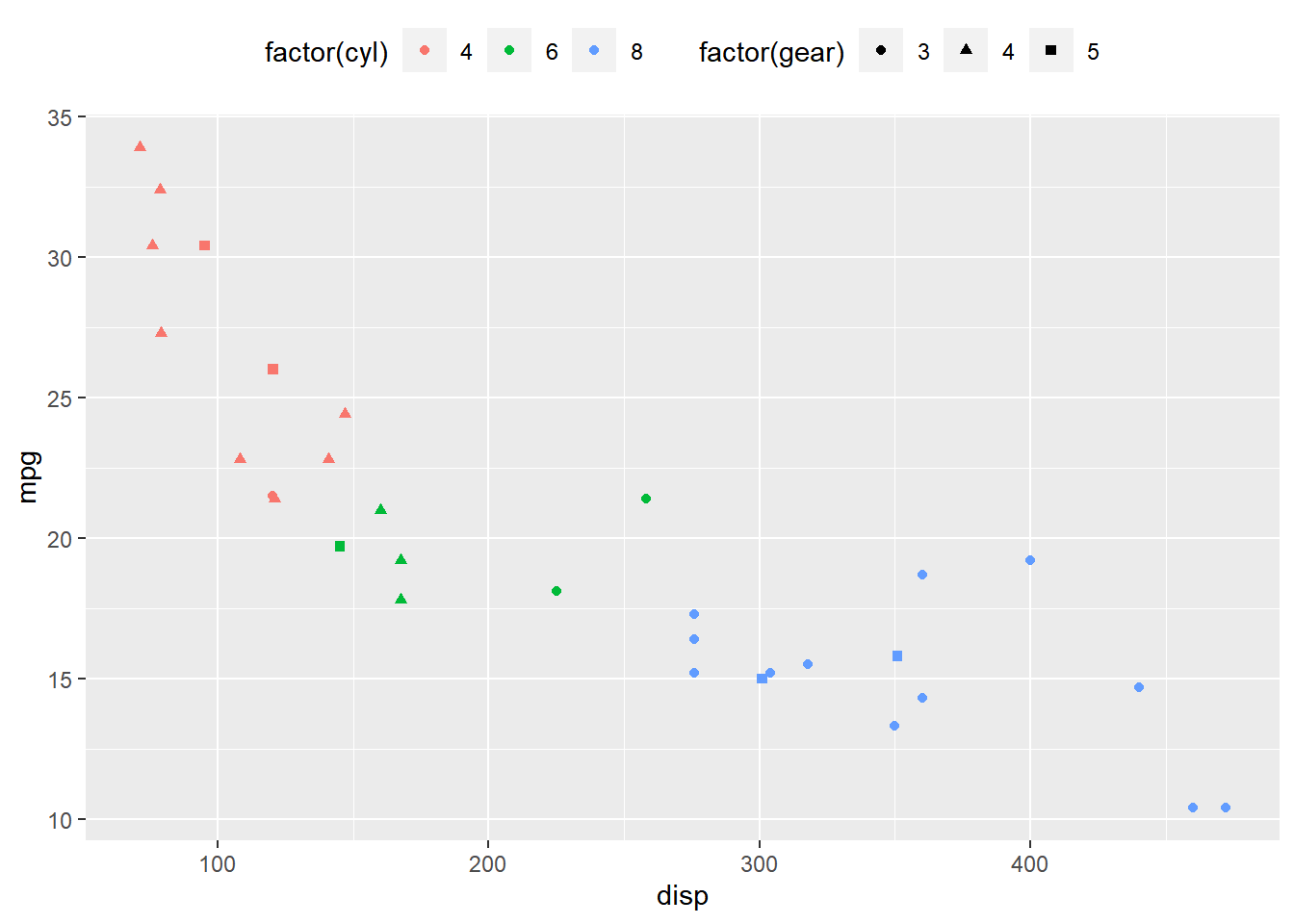
14.5 Themes
14.5.1 Classic Dark on Light
ggplot(mtcars) +
  geom_point(aes(disp, mpg)) +
  theme_bw()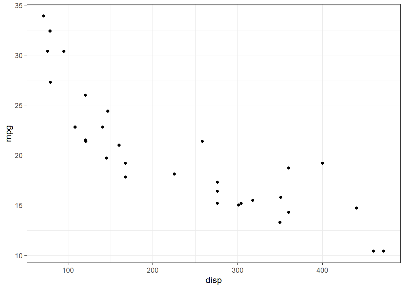
14.5.2 Default Gray
ggplot(mtcars) +
  geom_point(aes(disp, mpg)) +
  theme_gray()
14.5.3 Light
ggplot(mtcars) +
  geom_point(aes(disp, mpg)) +
  theme_light()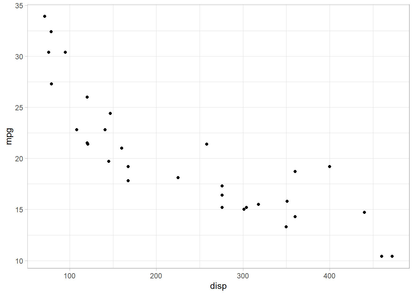
14.5.4 Minimal
ggplot(mtcars) +
  geom_point(aes(disp, mpg)) +
  theme_minimal()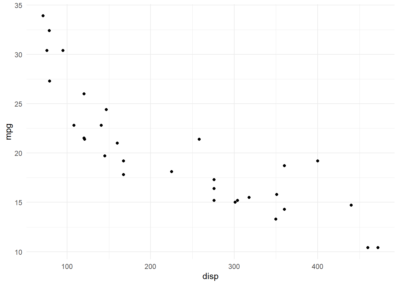
14.5.5 Dark
ggplot(mtcars) +
  geom_point(aes(disp, mpg)) +
  theme_dark()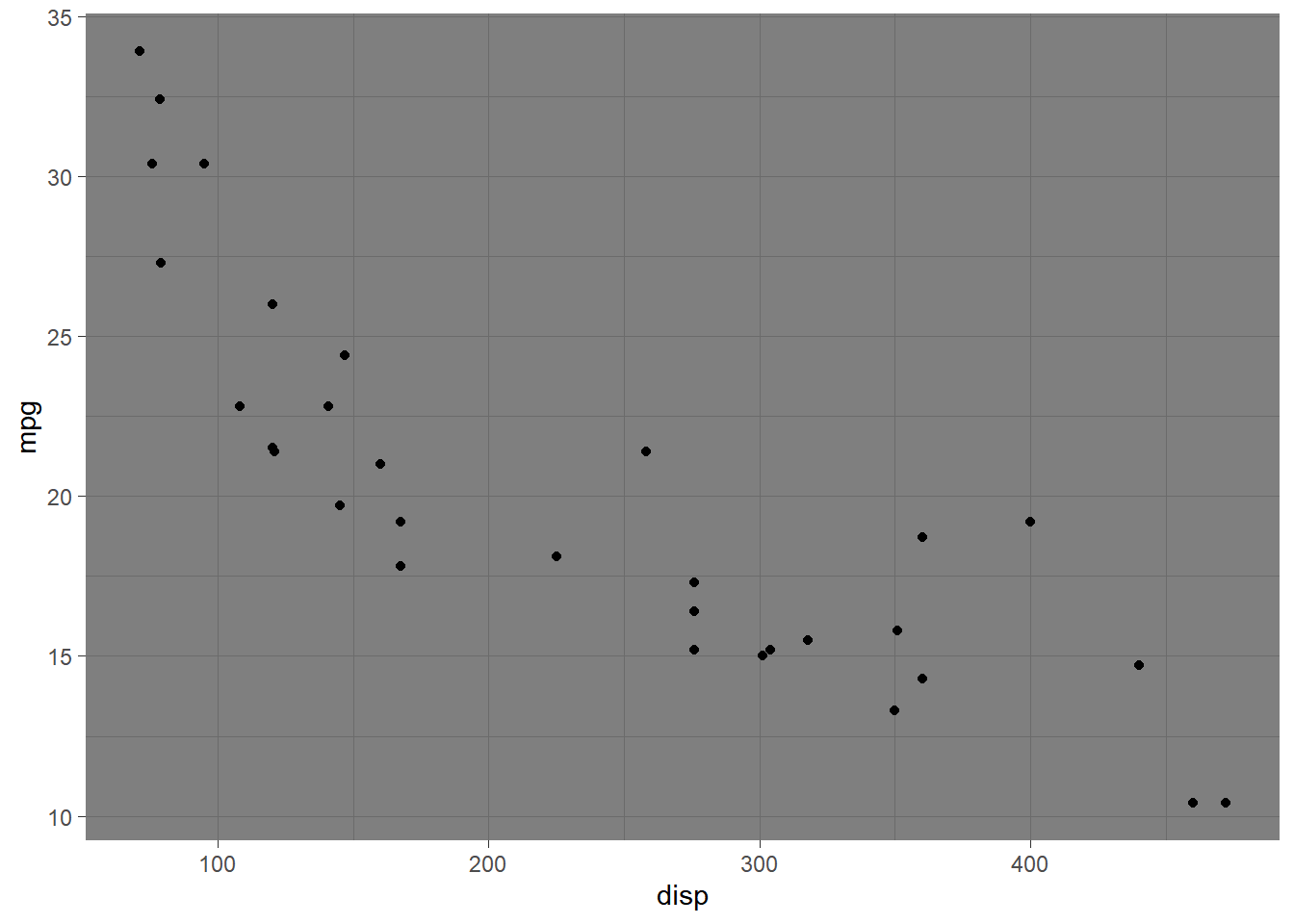
14.5.6 Classic
ggplot(mtcars) +
  geom_point(aes(disp, mpg)) +
  theme_classic()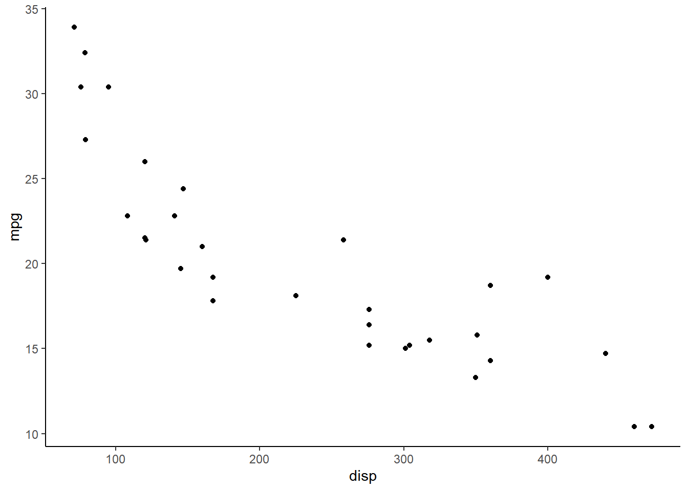
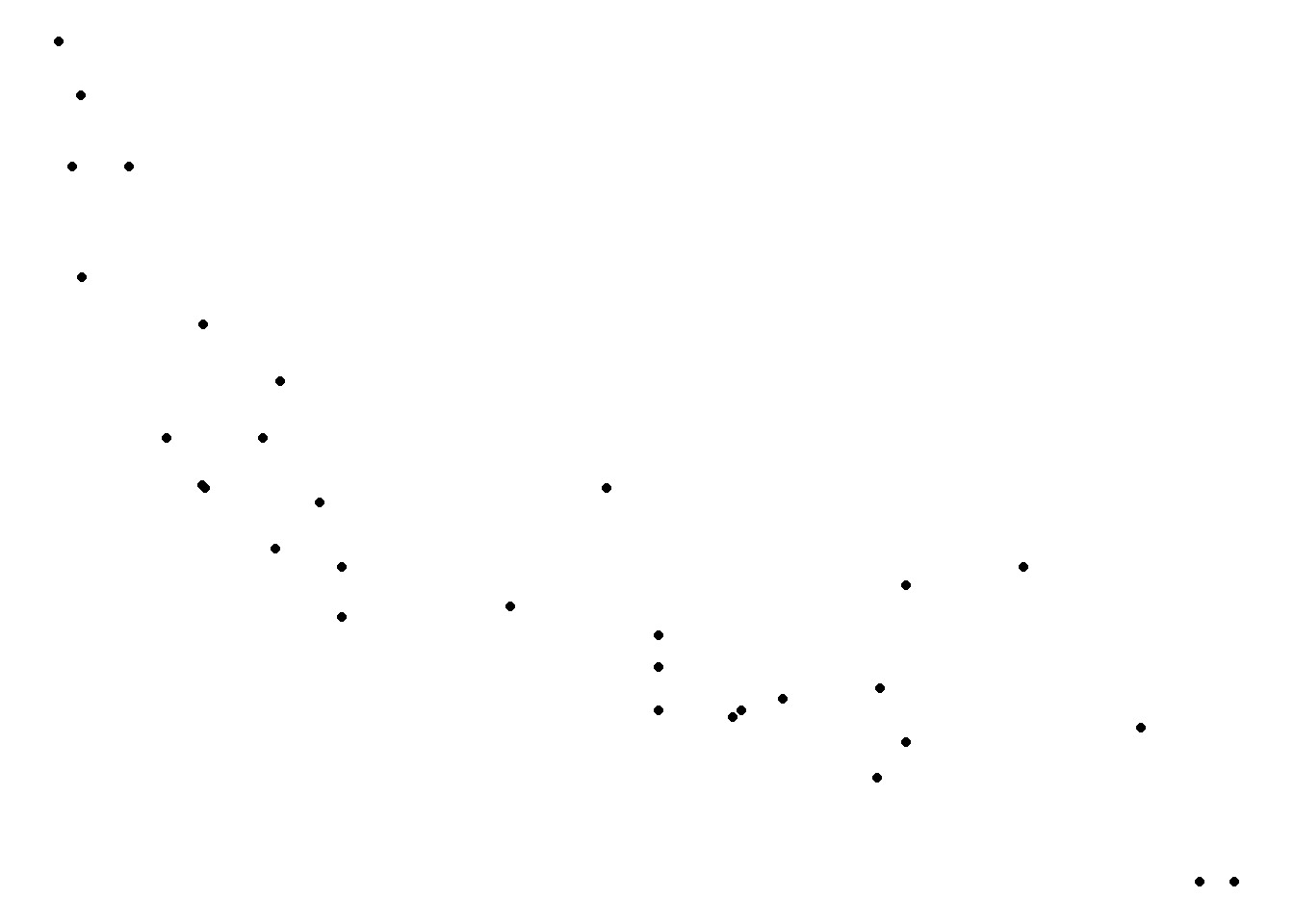
14.5.7 Void (Empty)
ggplot(mtcars) +
  geom_point(aes(disp, mpg)) +
  theme_void()