Chapter 13 Faceting
13.1 Introduction
In this chapter, we will learn about faceting i.e. combining plots.
Let us continue with the scatter plot examining the relationship between displacement and miles per gallon but let us make one additional change. We now want 3 sub plots for each type of cylinder. How can we do this? We can split or group the data by cylinder type and plot the subset of data which means dealing with 3 different data sets, plotting 3 plots and arranging them for comparison. ggplot2 offers the following 2 functions which allow us to plot subset of data with a simple formula based interface:
facet_grid()facet_wrap()
Faceting allows us to create multiple sub plots. It partitions a plot into a matrix of panels with each panel showing a different subset of data.
13.2 Grid
13.2.1 Vertical
facet_grid() allows us to split up the data by one or two discrete variables
and create sub plots. The sub plots can be arranged horizontally or vertically
using a formula of the form vertical ~ horizontal. In the below example, 3
sub plots are created, one each for the levels of the cyl variable and
the sub plots are arranged vertically
ggplot(mtcars, aes(disp, mpg)) +
  geom_point() +
  facet_grid(cyl ~ .)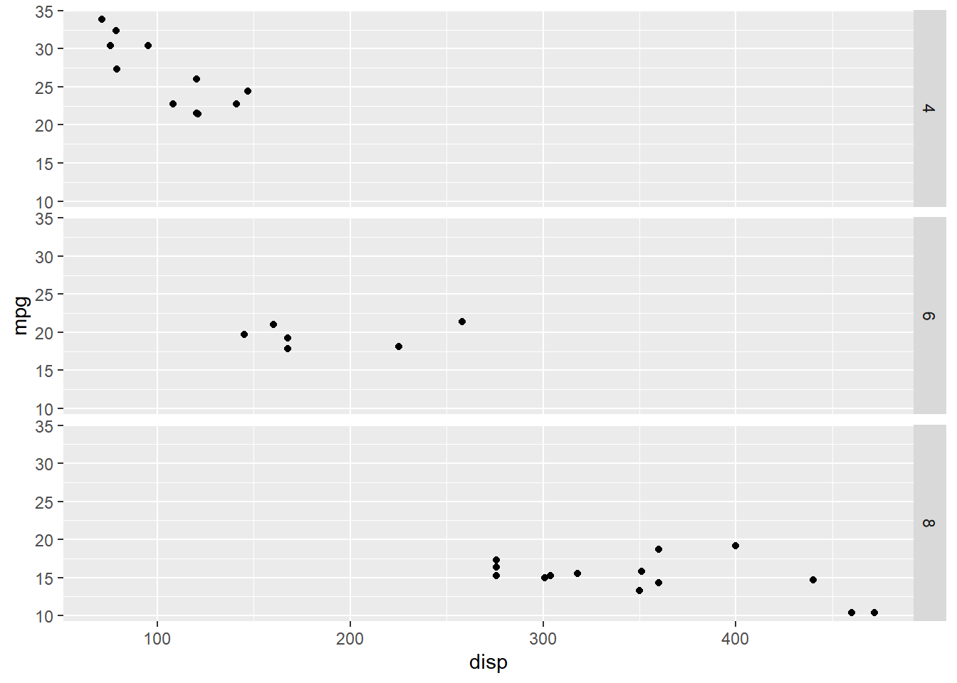
13.2.2 Horizontal
Below we reproduce the previous example but arrange the sub plots horizontally.
ggplot(mtcars, aes(disp, mpg)) +
  geom_point() +
  facet_grid(. ~ cyl)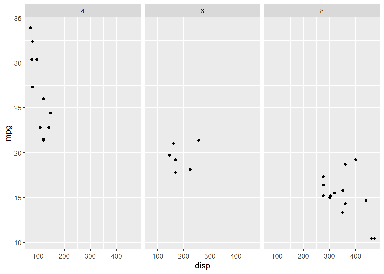
13.2.3 Vertical & Horizontal
In certain cases, we might want different discrete variables to represent the
horizontal and vertical direction. In the below example, we examine the
relationship between displacement and miles per gallon for different combinations
of cyl and gear variables.
ggplot(mtcars, aes(disp, mpg)) +
  geom_point() +
  facet_grid(cyl ~ gear)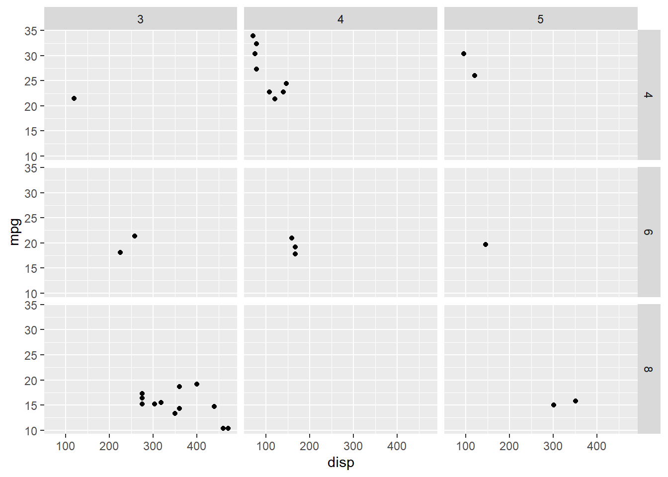
Below, we switch the variables representing the vertical and horizontal directions.
ggplot(mtcars, aes(disp, mpg)) +
  geom_point() +
  facet_grid(gear ~ cyl)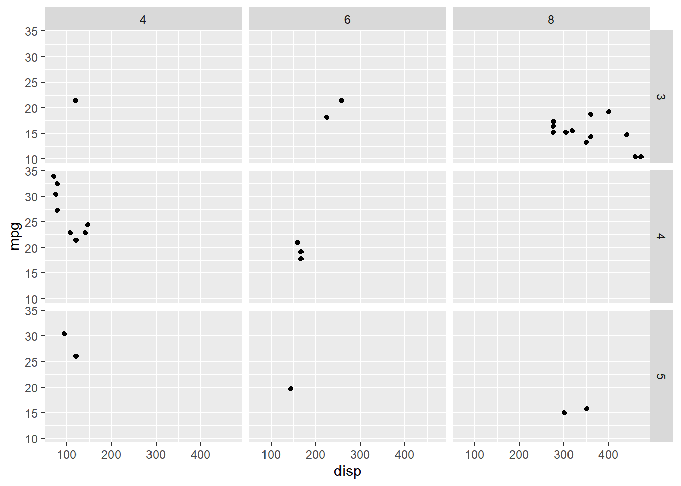
13.2.4 Scales
If you carefully observe the second example, the range of X axis is same for
all the 3 sub plots i.e. it is a fixed range. You can allow each of the sub
plots to have different range using the scales argument and supplying it the
value 'free'.
ggplot(mtcars, aes(disp, mpg, color = factor(cyl))) +
  geom_point() +
  facet_grid(. ~ cyl, scales = "free")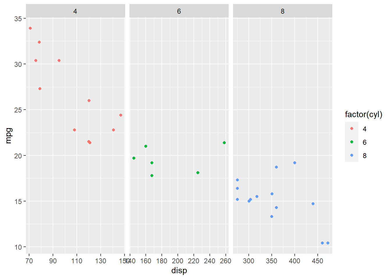
Now, each of the sub plot has a different range.
13.2.5 Switch Labels
In the third example, the labels are displayed at the bottom for X axis and
at the right for the Y axis. It can be changed using the switch argument
and supplying the value 'both'. The labels will now be displayed at the top
for the X axis and at left for the Y axis. If you just want to change the
labels for a particular axis, use the values x and y for the X and Y
axis respectively.
ggplot(mtcars, aes(disp, mpg)) +
  geom_point() +
facet_grid(cyl ~ gear, switch = "both") 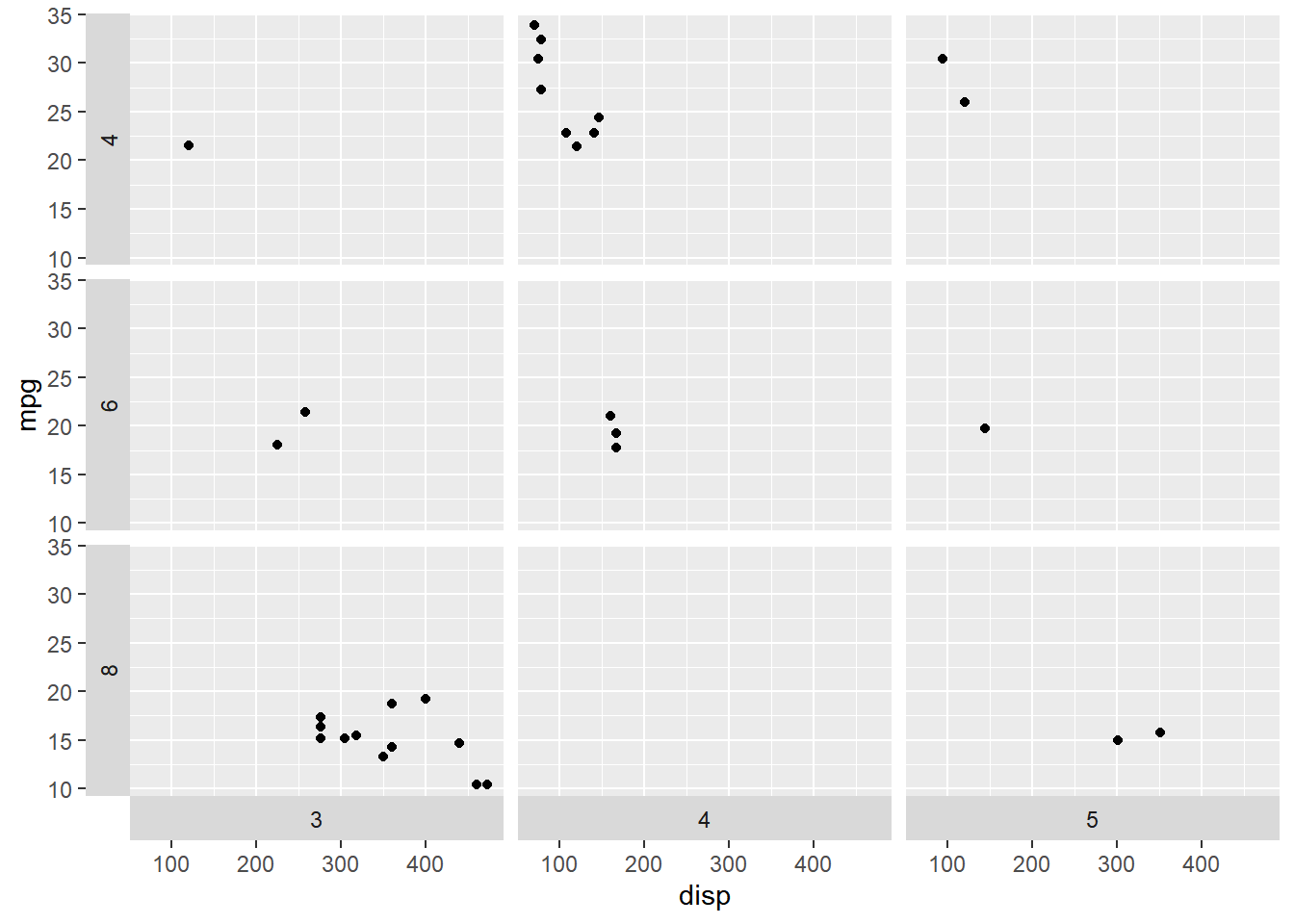
13.3 Wrap
facet_wrap() allows us to arrange sub plots in a certain number of rows and
columns. In the below example, we will use facet_wrap() to arrange the sub
plots in a single row.
ggplot(mtcars, aes(disp, mpg)) +
  geom_point() +
  facet_wrap(~cyl)
13.3.1 Specify Rows
To arrange the sub plots in a specific number of rows, use the nrow argument.
In the below example, we arrange the sub plots in 2 rows.
ggplot(mtcars, aes(disp, mpg)) +
  geom_point() +
  facet_wrap(~cyl, nrow = 2)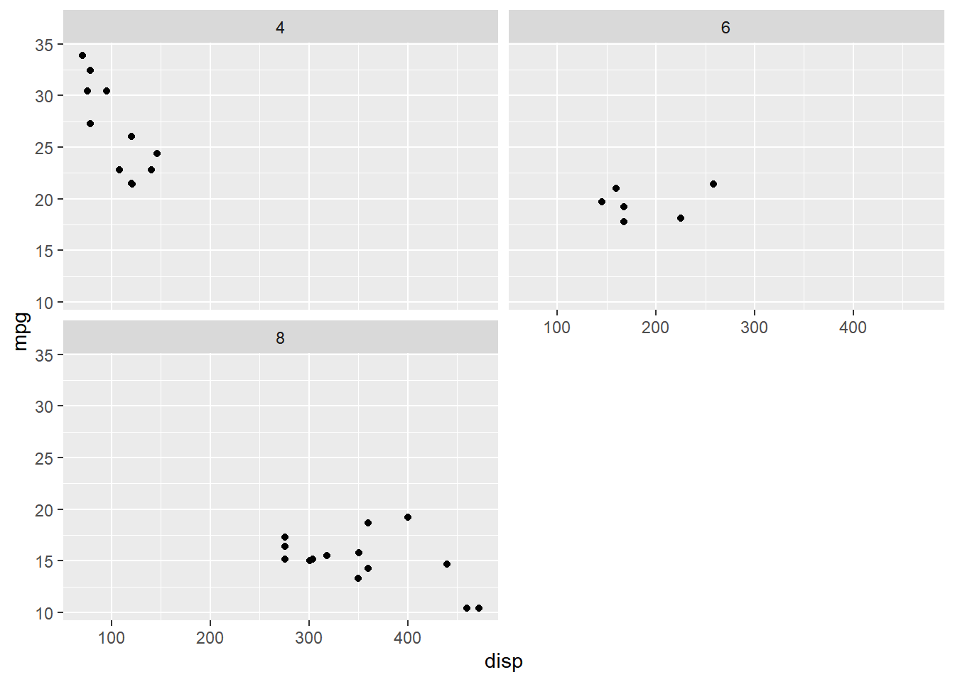
13.3.2 Specify Columns
Here, we arrange the sub plots in 3 columns instead of rows using the ncol
argument.
ggplot(mtcars, aes(disp, mpg)) +
  geom_point() +
  facet_wrap(~cyl, ncol = 3)
13.3.3 Scales
You can allow each of the sub plots to have different range using the scales
argument and supplying it the value 'free'.
ggplot(mtcars, aes(disp, mpg)) +
  geom_point() +
  facet_wrap(~cyl, scales = "free")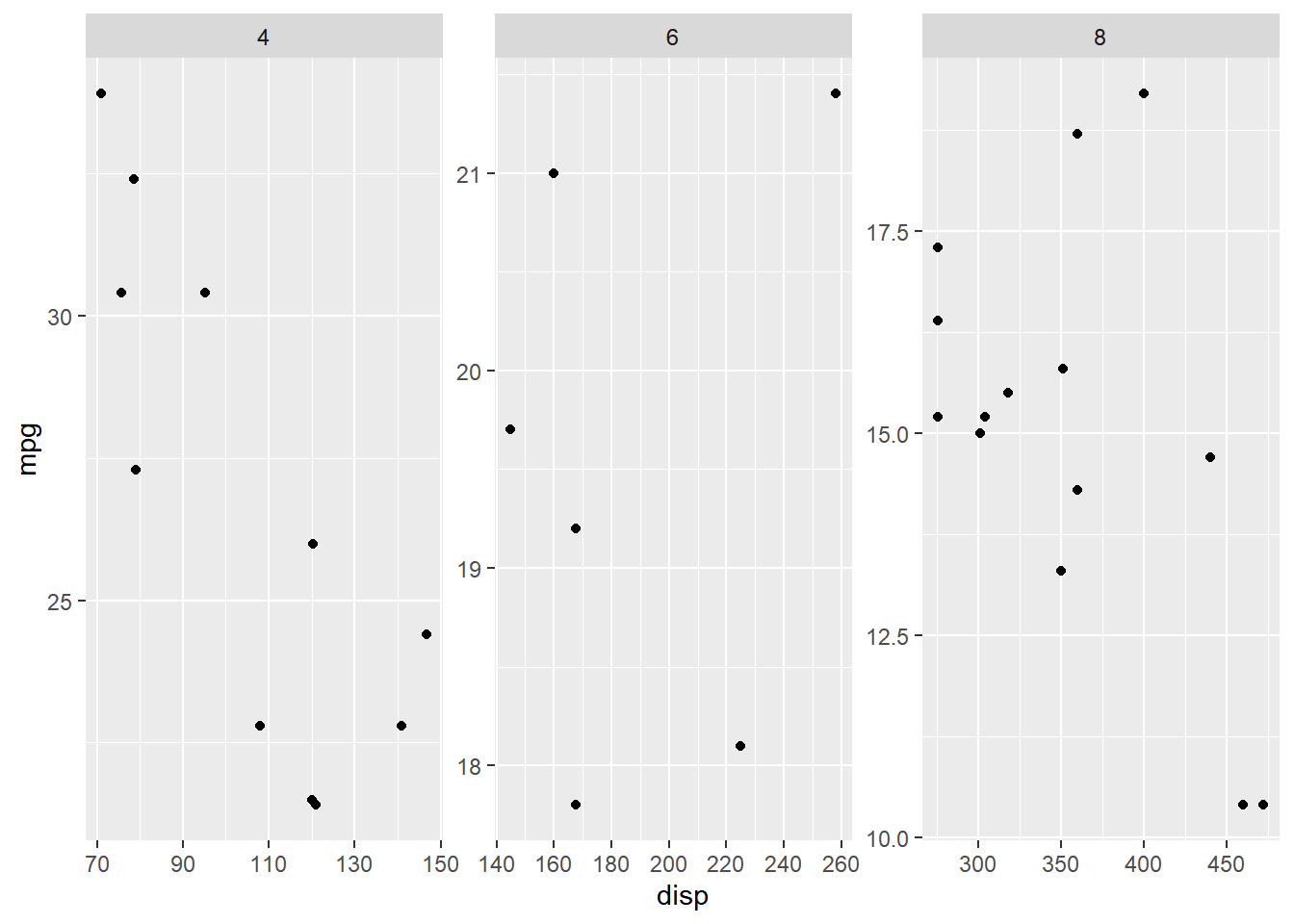
13.3.4 Rows & Columns
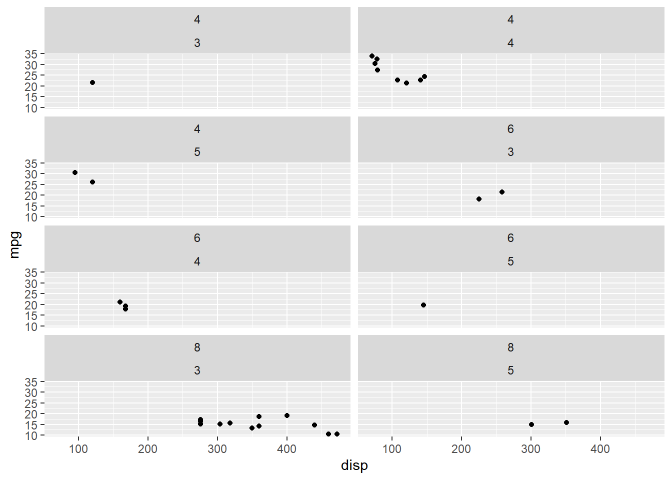
If 2 discrete variables are used to create the sub plots, we can either use the formula interface to specify the variables as shown below
ggplot(mtcars, aes(disp, mpg)) +
  geom_point() +
  facet_wrap(~cyl + gear, nrow = 2)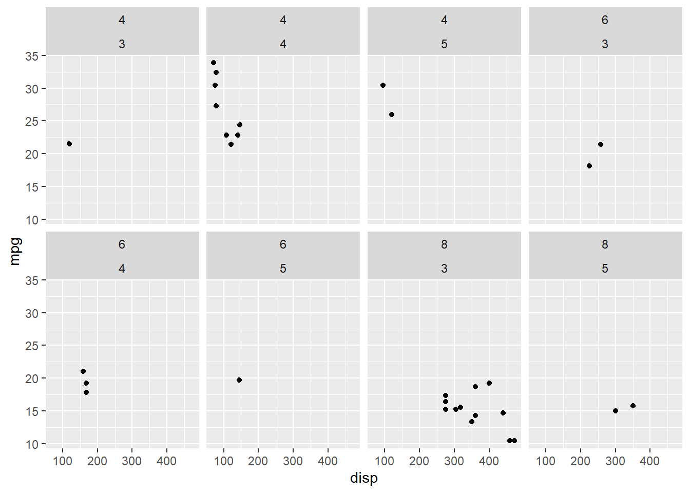
or use a character vector of variable names.
ggplot(mtcars, aes(disp, mpg)) +
  geom_point() +
  facet_wrap(c("cyl", "gear"), ncol = 2)